pingouin.plot_blandaltman

pingouin.plot_blandaltman(x, y, agreement=1.96, xaxis='mean', confidence=0.95, annotate=True, percentage=False, symmetric_ylim=False, ax=None, **kwargs)

Generate a Bland-Altman plot to compare two sets of measurements.

Parameters:

x, ypd.Series, np.array, or list

First and second measurements.

agreementfloat

Multiple of the standard deviation used to compute the limits of agreement (LoA). The default is 1.96, which gives LoA that contain approximately 95% of differences when they are normally distributed.

xaxisstr

Define which measurements should be used as the reference (x-axis). Default is to use the average of x and y (“mean”). Accepted values are “mean”, “x” or “y”.

confidencefloat or None

If not None, plot the specified confidence interval of the mean difference and limits of agreement. These bands represent sampling uncertainty around the point estimates (not prediction intervals): the larger the sample size, the narrower the bands. Default is 0.95.

annotatebool

If True (default), annotate the mean difference and upper/lower limits of agreement values on the right-hand side of the plot.

percentagebool

If True, plot percentage differences relative to the mean of each pair, i.e. (x - y) / abs(mean(x, y)) * 100. Useful when measurement variability scales with magnitude. This is only meaningful for ratio-scale measurements that stay away from zero: the percentage difference grows without bound as the mean of a pair approaches zero. Default is False.

Added in version 0.6.2.

symmetric_ylimbool

If True, force the y-axis to be symmetric around zero. This avoids conveying a visual bias when the mean difference is close to zero, but compresses the data into a narrow band when the bias is large relative to the spread of the differences. Default is False.

Added in version 0.6.2.

axmatplotlib axes

Axis on which to draw the plot.

**kwargsoptional

Optional argument(s) passed to matplotlib.pyplot.scatter().

Returns:

axMatplotlib Axes instance

Returns the Axes object with the plot for further tweaking.

Notes

Bland-Altman plots [1] are extensively used to evaluate the agreement among two different instruments or two measurements techniques. They allow identification of any systematic difference between the measurements (i.e., fixed bias) or possible outliers.

The mean difference (= x - y) is the estimated bias, and the SD of the differences measures the random fluctuations around this mean. If the mean value of the difference differs significantly from 0 on the basis of a 1-sample t-test, this indicates the presence of fixed bias. If there is a consistent bias, it can be adjusted for by subtracting the mean difference from the new method.

It is common to compute 95% limits of agreement for each comparison (average difference ± 1.96 standard deviation of the difference), which tells us how far apart measurements by 2 methods were more likely to be for most individuals. If the differences within mean ± 1.96 SD are not clinically important, the two methods may be used interchangeably. The 95% limits of agreement can be unreliable estimates of the population parameters especially for small sample sizes so, when comparing methods or assessing repeatability, it is important to calculate confidence intervals for the 95% limits of agreement. The standard error of the limits of agreement is √(3s²/n), per Bland & Altman (1986) [1].

The code is an adaptation of the PyCompare package. The present implementation is a simplified version; please refer to the original package for more advanced functionalities.

References

[1] (1,2)

Bland, J. M., & Altman, D. (1986). Statistical methods for assessing agreement between two methods of clinical measurement. The lancet, 327(8476), 307-310.

[2]

Giavarina, D. (2015). Understanding bland altman analysis. Biochemia medica, 25(2), 141-151.

Examples

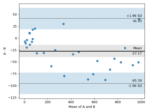
Bland-Altman plot (example data from [2])

>>> import pingouin as pg
>>> df = pg.read_dataset("blandaltman")
>>> ax = pg.plot_blandaltman(df["A"], df["B"])
>>> plt.tight_layout()